Frequentist vs Bayesian A/B Testing Thinking

The A/B Testing Concept

The A/B testing concept is fairly simple and widely known. At its core, it testing is about discovering which version performs better against a defined outcome.

Take a simple marketing example. Suppose a company is running an email campaign and wants to maximize clicks. They could split the list into two groups and test different send times — say, 9am vs 6pm. Whichever version produces more clicks reveals the better timing.

The Bayesian or Frequentist uses the same basic concept but with a flair of inferential statistics.

What is Inferential Statistics

Inferential Statistics takes information from a sample and uses it to make generalizations about a larger population. The purpose is to answer a specific question or test a hypothesis.

Let’s say we want to find the average height of males born in the USA. It would be nearly impossible to collect information on every single person. However, if we have a sample large enough, we can infer a conclusion with a certain level of confidence.

Frequentist Thinking in Plain Terms

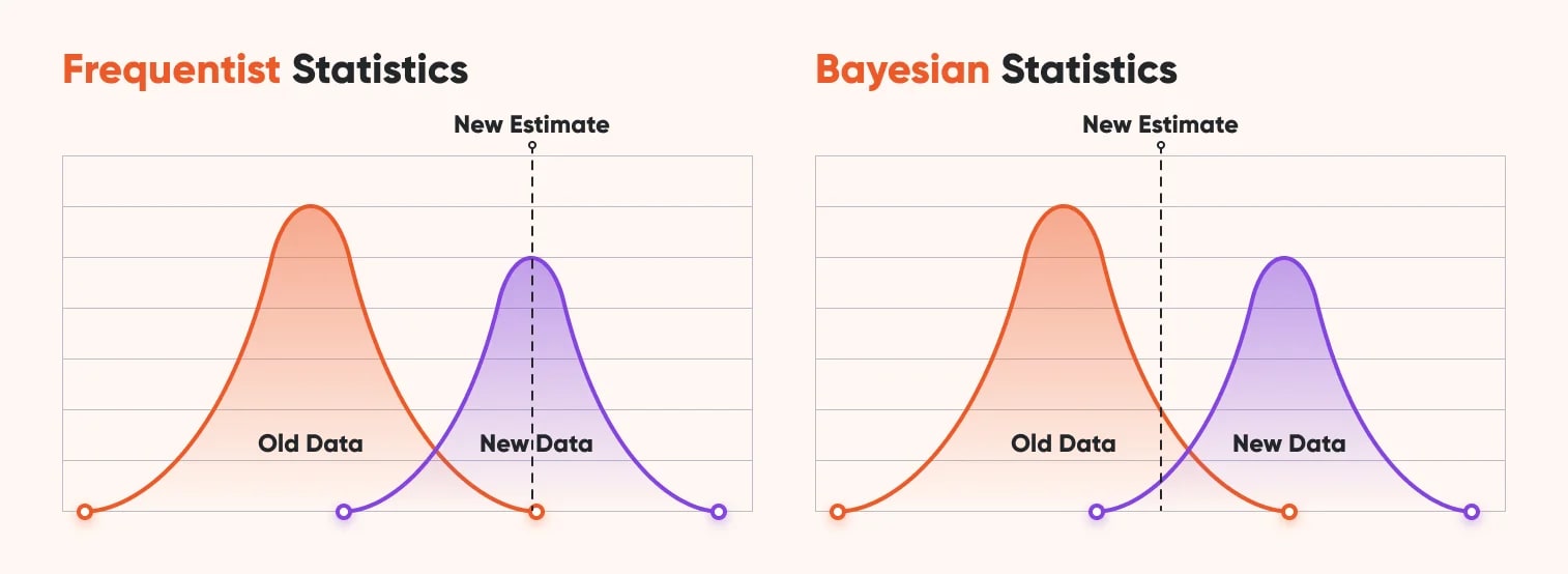
The Frequentist approach is the classic statistics you probably learned in school. It starts with the hypothesis that there is no difference between your options—like assuming that two coins are equally fair. But here’s the key question: if we ran the same experiment over and over again, how often would we see the difference just by chance?

Let’s break this down further. Consider two quarters—Quarter A and Quarter B. If you flip each 1,000 times, the results will very likely be different. Even if both coins were minted in the same batch and are nearly the same. To be frank, there is a very high change that you will get different numbers with the same coin.

This natural randomness is what frequentist statistics is designed to account for. It asks: If these coins were truly identical, and I repeated this exact experiment 100 times, how many of those times would I see a difference this just as big or smaller?

I could sit here and flip two coins a thousand times and collect the data. But that is not practical. To bring this to life, I wrote a little Python script to simulate two coins being flipped 1,000 times each:

import numpy as np

# Parameters
n_flips = 1000   # number of flips
p_heads = 0.5    # fair coin probability

# Simulate coin flips (0 = tails, 1 = heads)
flips_a = np.random.binomial(1, p_heads, n_flips)
flips_b = np.random.binomial(1, p_heads, n_flips)

# Count heads and tails for A
heads_count_a = np.sum(flips_a)
tails_count_a = n_flips - heads_count_a

# Counts heads and tails for B
heads_count_b = np.sum(flips_b)
tails_count_b = n_flips - heads_count_b

print(f"Total flips: {n_flips}")
print(f"Heads A: {heads_count_a}\nHeads B: {heads_count_b}")
print(f"Tails A: {tails_count_a}\nTails B: {tails_count_b}")

I ran it, and got these results:

Total flips: 1000
Heads A: 510
Heads B: 544
Tails A: 490
Tails B: 456

So, A landed heads 51% of the time, and B landed heads 54.4% of the time. That’s a 3.4% gap. The question is: is the gap real or just noise?

The Frequentist Math

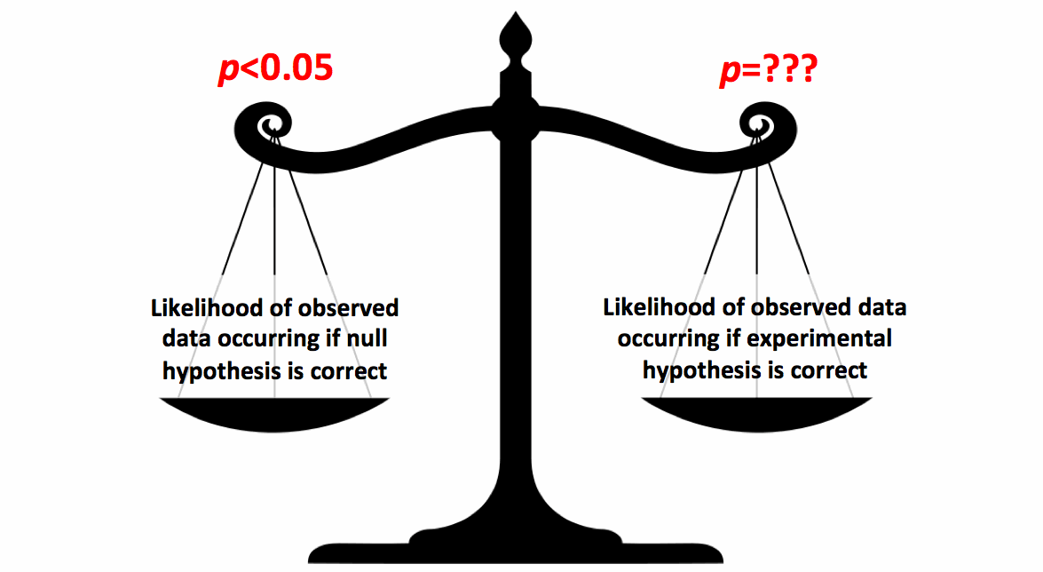
Here’s where the frequentist framework kicks in. It sets up a null hypothesis: the two coins are equally fair. We will now calculate how extreme the observed difference is under that assumption. That calculation produces our p-value.

Let’s look a little closer using math.

What It Means

At the common threshold of 0.05, we fail to reject the null hypothesis. In plain English: a 3.4% difference is not strong enough evidence — it could easily happen just by random chance.

That’s the Frequentist perspective. It doesn’t say, “There’s a 3.4% chance A and B are the same.” Instead, it says: “If they were the same, you’d expect to see a difference this large (or larger) about 13% of the time just by luck.”

Bayesian Approach

The Bayesian framework has a different approach. Instead of asking “how rare is this result if nothing’s different?” it asks: “given what I’ve observed, how likely is option A better than option B?”

The key idea is updating beliefs. You start with a prior belief (what you thought before collecting data), then add the new evidence, and end with a posterior belief.

Using the same example, let’s talk about the coins A and B. After flipping 1,000 times, we saw:

p̂_A = 0.510 (A’s proportion of heads)

p̂_B = 0.544 (B’s proportion of heads)

The frequentist says if these coins are exactly the same. The difference we saw is normal. This is likely to happen up to but not more than 13% of the time.

The Bayesian says something different. Given the results, there is a probability that coin B is actually better than A.

Conclusion

Frequentist and Bayesian approaches both tackle the same problem — making sense of uncertainty — but they frame the answer differently:

Frequentist:

If A and B were really the same, you’d expect to see a difference like this about 13% of the time.

Bayesian:

Given what we observed, there’s a 92% chance B is actually better than A.

Both are valid, and both have strengths and weaknesses. Either method can be right or wrong for your purposes.

Frequentist methods are widely used and mathematically rigorous, but the results can feel abstract. Bayesian methods, on the other hand, often provide a more intuitive story — probabilities you can act on — but they rely on priors, which can be subjective.

At the end of the day, business is still a gamble. But when you bring statistics into the picture, you move from guessing to making informed bets. A/B testing, powered by Frequentist or Bayesian inference, isn’t a crystal ball — but it can give you more confidence making decisions.