
FIELD NOTE · EDA
Creating Tables for Descriptive Analysis
When conduction EDA, multiple steps are required. When using python, other tools can be used to facilitate visualizations and other commands.
The first step in any data analysis is the discovery process. This is where we find the size, variable names, data types, and so on.
This is one of the most critical phase of the data analysis. Yet, it is the most tedious one. In the past, I’ve created steps different functions to automate some of the work.
The python ecosystem have tools that allow you to format DataFrames to give a more sophisticated look.
This comes handy for scholars when trying to create Tables for research papers. For desmonstration purposes, I used the Palmer Penguins dataset. I did not do any statistical analysis, this was for EDA purposes only.
Loading the Data
First, we need to install all of the packages we are going to use for this project. Note, some of these packages have changed names over time, and are likely to do again. If you are having trouble downloading one, you can always check out the PyPi website.
%pip install pandas seaborn skimpy tailbone great-tables fg-data-profiling
We can load the data from seaborn.
import pandas as pd
import seaborn as ins

df = sns.load_dataset("penguins")
After so many years doing this, the next commands have become almost a second nature.
print(df.shape)
print(df.dtypes)
print(df.isna().sum())
Getting the Baseline
We all know that Python has the built-in describe() function. That’s a good starting point.
df.describe().round(2)
This command is not very complete. It is missing several critical elements that would require me to run several other commands to get a full picture. For instance, it doesn’t have skewness or kurtosis.
Don’t get me wrong, pandas is more than capable to show us all of that information. With couple other commands, you can get more information from the data.
df.describe(include="all").round(2)
It provides a better output, but still not enough information. The looks of the table is not the best either. By the way, I hate when my tables have NaN.
We can also build a summary with .agg(). That comes handy when you want to control the statistics.
numeric = df.select_dtypes("number")
summary = numeric.agg(["mean", "median", "std", "skew", "kurt"]).T
summary["missing_pct"] = df[numeric.columns].isna().mean().mul(100).round(1)
summary.round(2)
That gives you a little more information and it is customizable. You can also use the .groupby() function, which will also provide a summary based on the specie of the penguin.
df.groupby("species")["body_mass_g"].describe().round(1)
Getting a More Robust Summary with skimpy
Skimpy is a supercharged describe(). It handles every column at once and it generates a nice report.
from skimpy import skim

skim(df)
Output:
╭─────────────────────────────────────────────────── skimpy summary ───────────────────────────────────────────────────╮
│          Data Summary                Data Types                                                                      │
│ ┏━━━━━━━━━━━━━━━━━━━┳━━━━━━━━┓ ┏━━━━━━━━━━━━━┳━━━━━━━┓                                                               │
│ ┃ Dataframe         ┃ Values ┃ ┃ Column Type ┃ Count ┃                                                               │
│ ┡━━━━━━━━━━━━━━━━━━━╇━━━━━━━━┩ ┡━━━━━━━━━━━━━╇━━━━━━━┩                                                               │
│ │ Number of rows    │ 344    │ │ float64     │ 4     │                                                               │
│ │ Number of columns │ 7      │ │ string      │ 3     │                                                               │
│ └───────────────────┴────────┘ └─────────────┴───────┘                                                               │
│                                                       number                                                         │
│ ┏━━━━━━━━━━━━━━━━━━━━━┳━━━━━┳━━━━━━━━━━━━━━━━━━━━━┳━━━━━━━━┳━━━━━━━━┳━━━━━━┳━━━━━━━┳━━━━━━━┳━━━━━━┳━━━━━━┳━━━━━━━━┓  │
│ ┃ column              ┃ NA  ┃ NA %                ┃ mean   ┃ sd     ┃ p0   ┃ p25   ┃ p50   ┃ p75  ┃ p100 ┃ hist   ┃  │
│ ┡━━━━━━━━━━━━━━━━━━━━━╇━━━━━╇━━━━━━━━━━━━━━━━━━━━━╇━━━━━━━━╇━━━━━━━━╇━━━━━━╇━━━━━━━╇━━━━━━━╇━━━━━━╇━━━━━━╇━━━━━━━━┩  │
│ │   bill_length_mm    │   2 │  0.5813953488372093 │  43.92 │   5.46 │ 32.1 │ 39.23 │ 44.45 │ 48.5 │ 59.6 │ ▃█▆█▃  │  │
│ │    bill_depth_mm    │   2 │  0.5813953488372093 │  17.15 │  1.975 │ 13.1 │  15.6 │  17.3 │ 18.7 │ 21.5 │ ▄▅▆█▆▂ │  │
│ │  flipper_length_mm  │   2 │  0.5813953488372093 │  200.9 │  14.06 │  172 │   190 │   197 │  213 │  231 │ ▂██▄▆▃ │  │
│ │     body_mass_g     │   2 │  0.5813953488372093 │   4202 │    802 │ 2700 │  3550 │  4050 │ 4750 │ 6300 │ ▂█▆▄▃▁ │  │
│ └─────────────────────┴─────┴─────────────────────┴────────┴────────┴──────┴───────┴───────┴──────┴──────┴────────┘  │
│                                                       string                                                         │
│ ┏━━━━━━━━━┳━━━━┳━━━━━━━━━━━━━┳━━━━━━━━━━┳━━━━━━━━━━━┳━━━━━━━━┳━━━━━━━━━━━┳━━━━━━━━━━━━━┳━━━━━━━━━━━━━┳━━━━━━━━━━━━┓  │
│ ┃         ┃    ┃             ┃          ┃           ┃        ┃           ┃ chars per   ┃ words per   ┃ total      ┃  │
│ ┃ column  ┃ NA ┃ NA %        ┃ shortest ┃ longest   ┃ min    ┃ max       ┃ row         ┃ row         ┃ words      ┃  │
│ ┡━━━━━━━━━╇━━━━╇━━━━━━━━━━━━━╇━━━━━━━━━━╇━━━━━━━━━━━╇━━━━━━━━╇━━━━━━━━━━━╇━━━━━━━━━━━━━╇━━━━━━━━━━━━━╇━━━━━━━━━━━━┩  │
│ │ species │  0 │           0 │  Adelie  │ Chinstrap │ Adelie │  Gentoo   │        6.59 │           1 │        344 │  │
│ │ island  │  0 │           0 │  Dream   │ Torgersen │ Biscoe │ Torgersen │        6.09 │           1 │        344 │  │
│ │   sex   │ 11 │ 3.197674418 │   Male   │  Female   │ Female │   Male    │        4.99 │        0.97 │        333 │  │
│ │         │    │      604651 │          │           │        │           │             │             │            │  │
│ └─────────┴────┴─────────────┴──────────┴───────────┴────────┴───────────┴─────────────┴─────────────┴────────────┘  │
╰──────────────────────────────────────────────────────── End ─────────────────────────────────────────────────────────╯
That’s a much nicer report.
Generating a Full Interactive Report with Profiling
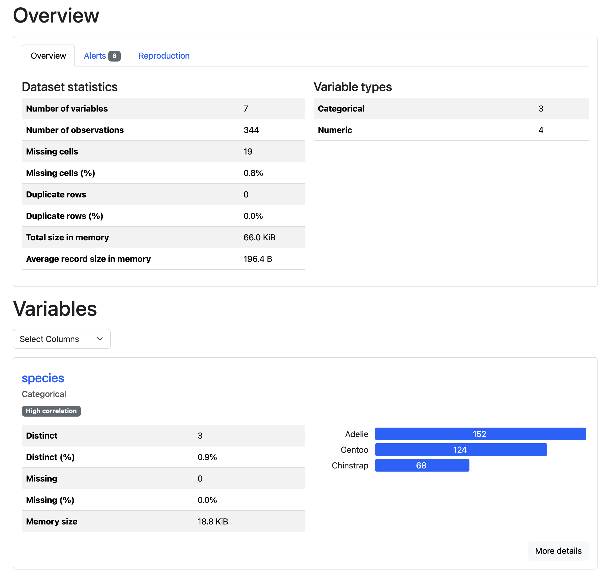
Now, when you need something that will provide you a full picture, data-profiling will provide you that.
from data_profiling import ProfileReport
profile = ProfileReport(df, title="Penguins Profiling Report", explorative=True)
Conclusion
Using this function, can cut down on some time you spend running commands. I don’t consider this an automation as you still need to run multiple commands. It does help, however with visualization and nice looking tables.