
Why is Central Tendency Important? Why Do We Use It?
Central tendency is one of the basic tools to help us understand essential information about the values of a dataset.
You are out and about with a large group of friends. Suddenly, everyone is hungry. As a group, you take a vote to decide if you are going to restaurant A or B.
The majority of your friends, decided on restaurant B. And that’s where everyone goes.
In a simple way, you are measuring central tendency. A task so mundane, it goes unnoticed. For a research, where the data is collected much larger than a group of friends, summarizing the frequency into categories becomes critical.
What is Central Tendency
Technically, central tendendy is defined as “the statistical measure that identifies a single value as representative of an entire distribution.” The idea, although not always the case, is to provide a description of the entire data.
It enables researchers to make general statements about the data. The mean, median, and mode are the three most common measures of central tendency.
Each of these measures have an unique function and reflect a different aspect of the data center.
Mean
The mean is commonly used measure used of central tendency.
During the World Cup games last month, central tendency was often used to describe the age of the teams on the pitch.
For instance, on the game Norway vs Brazil, in the round of 16, the commentators described the Noregian team being younger than their adversary. A fact, I later confirmed. The five-time champion’s team was sitting at 28.55 and the Scandinavian was at 26.34. A little over two years younger.
The mean is most appropriate when the data are normally distributed and when there is no significant outliers. That doesn’t mean you cannot calculate the mean for a non-normal data.
In such cases, it becomes less representative of the “typical” observation. It doesn’t mean that you cannot use it. Let’s look at the Brazilian National Team distribution.
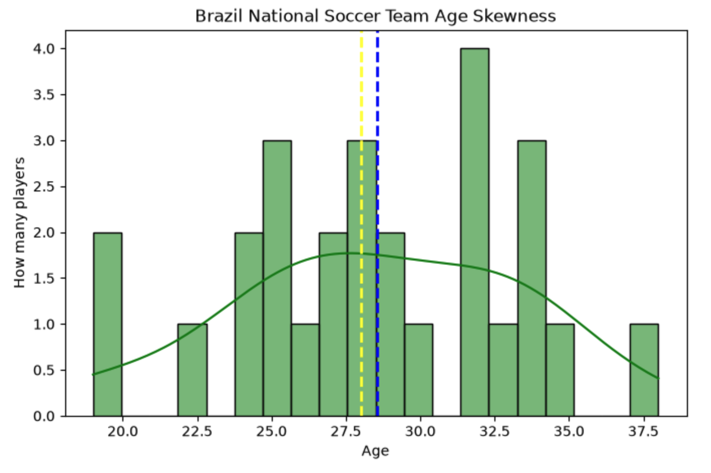
The age doesn’t appear to be normally distributed. We can see gaps and the largest number of players are 32 years old, well above the mean of 28.55. However, the median and mean line are really close, indicating limited skewness.
It doesn’t stop us from accurately determining that the Brazilian team was older than its adversary.
The Median
The Median is the middle value in the dataset. The median is the average between the two middle values.
Unlike the mean, outliers don’t affect the median, making it a more robust measure when dealing with skewed distributions.
The median is useful when the data are not symmetric distributed or when extreme values are present. In which case, it provides a more appropriate representation of the “typical” in the dataset.
In real estate, the “average” price of a house is measured with the median. Because it best represents the median price of a home in that specific location.
Here are the market values of homes in a section of the city:
Home 1: $250,000
Home 2: $275,000
Home 3: $300,000
Home 4: $325,000
Home 5: $5,000,000
Noticed that the outlier is extreme. If we are to take the mean, the price would be $1,230,000. The mean makes the neighborhood look expensive. Then you drive around and see that most house are one story ranch.
That price doesn’t represent any actual homes in the list.
Thus, the more appropriate would be the median: $300,000.
The Mode
The mode is the value that occurs most frequently in a dataset. It can be used to determine the most common category or response.
This measurement is especially useful in nominal data to identify the most frequently occurring category.
A shoe store trying to determine the most sold size. Keep in mind that a shoe size, while a number, it is categorical data. The mean could land on 8.94. That’s not a shoe size.
The most common size, could be a 9, and it appeared 100 times in a large dataset. Now, the store owner knows what size to restock.
No comments yet. Be the first.